Automating Knowledge Graph Creation with Gemini and ApertureDB – Part 4

From Semantic Layer → End-to-End Q&A and Comprehensive Evaluation 

Recap & Objectives

So far we have extracted entities, properties, and relationships from a PDF corpus, ingested them into ApertureDB, generated 768-dim Gemini embeddings for every entity, stored them in a DescriptorSet, and wired each vector to its source node via has_embedding.

We can now test two Retrieval-Augmented Generation pipelines:

This part shows how to build both pipelines and, importantly, why evaluating them is more nuanced than tossing Precision@k, Recall@k and MAP at the problem.

Notebook & Data: As before, code below is trimmed for readability. The full, executable Colab notebook (with setup cells, error handling, logging, etc.) and the complete Github repo are linked. The repo also contains some sample data you can use to run the notebooks. You will find that there are two versions of the notebook:

• The cloud version involves signing up on ApertureDB Cloud and configuring your instance there for a persistent, managed database.
• The local udocker version involves setting up the DB instance locally using udocker (which allows running Docker containers in constrained environments like Colab notebooks) - no sign-up needed. However, your data doesn’t persist unless you actually save it somewhere locally.

Aside from this DB set-up aspect, the notebooks are exactly similar so feel free to follow whichever suits you best.

‍

Building the Retrieval Building Blocks

Semantic Entry Points (shared by both pipelines)

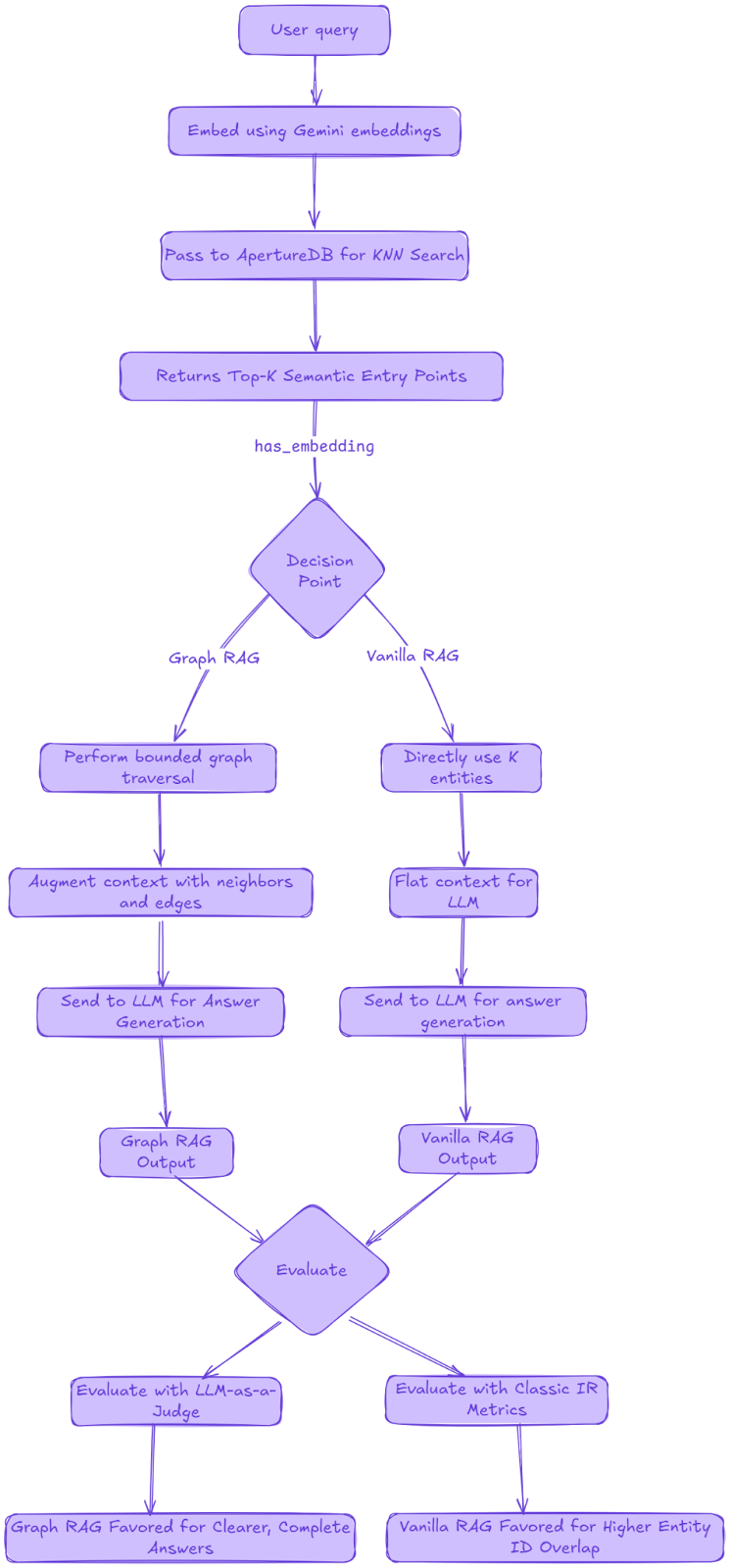
We embed the user query with Gemini, pass that vector into ApertureDB’s K-NN search on entity_embeddings_gemini, and immediately walk the has_embedding edge to surface the linked entities - all in one JSON query. ApertureDB’s integration with LlamaIndex and LangChain further facilitate RAG operations.

‍

def find_semantic_entry_points(query: str, k: int) -> list[dict]:
    # 1. embed the query
    cfg = types.EmbedContentConfig(
        output_dimensionality=EMB_DIMS,
        task_type="QUESTION_ANSWERING",
    )
    vec = gemini_client.models.embed_content(
        model=GEMINI_MODEL,
        contents=[query],
        config=cfg,
    ).embeddings[0].values
    vec_bytes = np.array(vec, dtype=np.float32).tobytes()


    # 2. chained ApertureDB query
    q = [
        {"FindDescriptor": {
             "set": DESCRIPTOR_SET,
             "k_neighbors": k,
             "distances": True,
             "_ref": 1}},
        {"FindEntity": {        # hop through has_embedding
             "is_connected_to": {"ref": 1, "connection_class": "has_embedding"},
             "results": {"all_properties": True}}},
    ]
    resp, _ = client.query(q, [vec_bytes])


    descriptors = resp[0]["FindDescriptor"]["entities"]
    entities    = resp[1]["FindEntity"]["entities"]
  # enrich entities with their class for downstream formatting
    class_map = {d["source_entity_id"]: d["source_entity_class"] for d in descriptors}
    for e in entities:
        e["class"] = class_map.get(e["id"], "Unknown")
    return entities

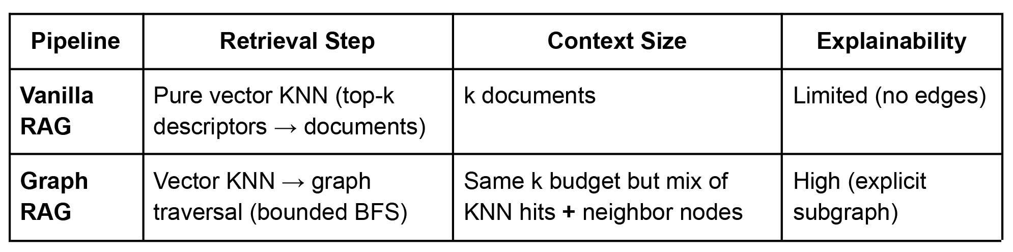
‍Pipeline A – Vanilla RAG
‍

def vanilla_rag(query: str, k: int) -> str:
    entities = find_semantic_entry_points(query, k)
    return "\n\n".join(pretty_props(e) for e in entities)

‍That’s literally it: pure vector search. Fast, simple, opaque.

Pipeline B – Graph RAG

Graph RAG augments the same vector search with a breadth-first “context bloom”:

1. Start with the k semantic entry points.
   
   
2. Traverse up to h hops, collecting new nodes until we hit a max_entities budget.
   
   
3. Deduplicate and stringify entities and edges for the LLM.
   
   

Below is the trimmed essence (full version in the notebook):

‍

def build_graph_context(entry_entities, max_hops=2, max_entities=20):
    frontier = {e['id'] for e in entry_entities}
    explored = set(frontier)
    context  = [pretty_props(e) for e in entry_entities]


    for _ in range(max_hops):
        if len(explored) >= max_entities: break
        next_frontier = set()


        # batch query for edges around current frontier
        q = []
        for i, eid in enumerate(frontier, 1):
            cls = next(e['class'] for e in entry_entities if e['id'] == eid)
            q += [
                {"FindEntity":    {"with_class": cls, "constraints": {"id": ["==", eid]}, "_ref": i}},
                {"FindConnection":{"src": i, "results": {"all_properties": True}}},
                {"FindConnection":{"dst": i, "results": {"all_properties": True}}}
            ]
        resp, _ = client.query(q)


        # parse edges, discover new node IDs
        new_ids = set()
        for block in resp:
            if "FindConnection" not in block: continue
            for conn in block["FindConnection"].get("connections", []):
                new_ids |= {conn["src_id"], conn["dst_id"]}


        new_ids -= explored
        if not new_ids: break


        # fetch their properties
        fetch = [{"FindEntity": {"constraints": {"id": ["in", list(new_ids)]},
                                 "results": {"all_properties": True}}}]
        ents, _ = client.query(fetch)
        for e in ents[0]["FindEntity"]["entities"]:
            e["class"] = e.get("class", "Unknown")  # filled server-side if schema present
            context.append(pretty_props(e))
            explored.add(e["id"])
            if len(explored) >= max_entities: break
        frontier = new_ids
    return "\n".join(context)

A convenience wrapper ties the pieces together:

‍

def graph_rag(query: str,
              k_start=3,
              max_hops=2,
              max_entities=20) -> str:
    start_entities = find_semantic_entry_points(query, k_start)
    return build_graph_context(start_entities, max_hops, max_entities)

‍Quick Side-by-Side Demo

Let’s fire a domain-specific question at both pipelines:

‍

q = "What does a hypervisor actually do?"


ctx_graph   = graph_rag(q, k_start=3, max_entities=20)
ctx_vanilla = vanilla_rag(q, k=20)


ans_graph   = gemini_client.models.generate_content(
                 model="gemini-2.5-flash",
                 contents=f"Use this context to answer:\n\n{ctx_graph}\n\nQ: {q}\nA:"
              ).text


ans_vanilla = gemini_client.models.generate_content(
                 model="gemini-2.5-flash",
                 contents=f"Use this context to answer:\n\n{ctx_vanilla}\n\nQ: {q}\nA:"
              ).text

‍Graph RAG context (excerpt):
‍

Entity: 'Hypervisor' (Class: 'Hypervisor', ID: 223)
 - definition: a software layer that allows multiple virtual machines...


Entity: 'Virtualization' (Class: 'Virtualization Technology', ID: 95)
 - benefit: optimizes computing power, storage, and network resources


 - [Hypervisor] --(runs_on)--> [Compute Node]
 - [Virtualization] --(enables)--> [Cloud Computing]
...

‍Explainability: An Important Benefit of Graph RAGWe can visualise the inner workings of graph RAG by mapping out the exact subgraph used for context generation. This overcomes the opaqueness aspect of Vanilla RAG. (Please refer to the notebook for a clearer depiction of the subgraph).

Entity: 'Hypervisors' (Class: 'Software', ID: 200)
  - function: manage VM isolation
  - vm_execution_management: manage VM isolation


Entity: 'Device Mediation & Access Control' (Class: 'Concept', ID: 71)
  - characteristics: Hypervisors emulate hardware devices, allowing VMs to interact with peripherals.
  - definition: Hypervisors emulate hardware devices, allowing VMs to interact with peripherals.
...

Notice the extra relational breadcrumbs (runs_on, enables, etc.). In contrast, the vanilla context is a flat list of entities with no linkage.

Generated answers: ‍

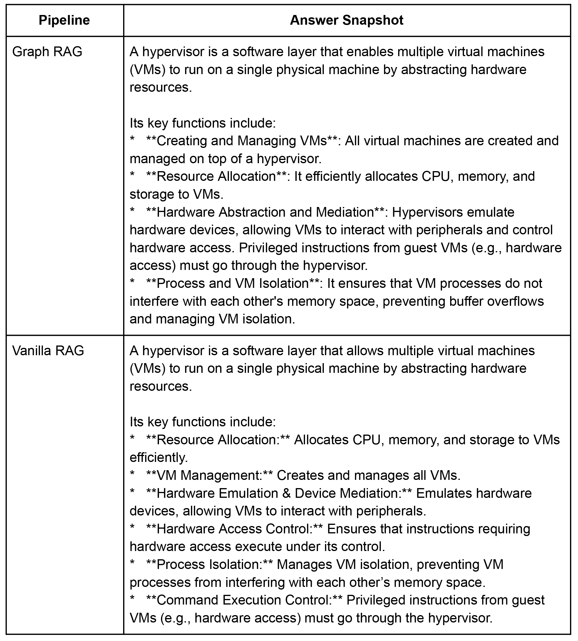
I asked two reasoning LLMs (Gemini-2.5-pro and GPT-o3) which answer was better in terms of relevance and accuracy and they both preferred the Graph RAG answer due to better organisation, conciseness and clarity (see for yourself in the notebook). But this isn’t enough; we need a systematic evaluation. 

Benchmarking the Two Pipelines – First Pass: Classic IR Metrics

I started with the usual retrieval-quality trio - Precision@k, Recall@k, and MAP - on a mini bench of ten domain questions which I generated using Gemini 2.5 pro by providing it the entities’ documents we curated in Part 1.
For each query I prepared a gold set of fifteen ideal entity IDs (again this was done by providing Gemini 2.5 Pro the eval queries and the contextual docs in the DB). Both pipelines were constrained to return at most fifteen entities per query so the playing field was level.

Outcome

• Vanilla RAG hit 0.64 on both precision and recall, and ≈ 0.57 MAP.
  
  
• Graph RAG landed at ≈ 0.43 on both precision and recall, and ≈ 0.38 MAP.
  

At face value vanilla RAG “wins”. Why? Because these metrics only reward ID overlap: the closer a retrieved list is to the gold IDs, the better the score. A pure vector top-k strategy is tailor-made for maximising that overlap, whereas Graph RAG deliberately trades a portion of semantic similarity for structural relevance; it drags in neighbours that expand context even if they sit a little farther away in embedding space. Classic IR metrics simply cannot see the value in those extra nodes. (When to use Graphs in RAG: A Comprehensive Analysis for Graph Retrieval-Augmented Generation)

‍Hidden Costs These Metrics Ignore

• Latency & Cost: Graph traversal is index-free and near-zero-latency, while every extra vector hit forces a high-dimensional ANN search.
  
  
• Explainability: Edges provide provenance; vectors do not.
  
  
• Generation Quality : Ultimately we care about the answer paragraphs, not the overlap score.
  

A Second Pass: LLM-as-a-Judge

To measure actual answer quality I ran an LLM-v-LLM bake-off:

1. For each query, both pipelines produced a context capped at 15 entities/documents.
   
   
2. Gemini 2.5 Flash generated an answer from that context.
   
   
3. Gemini 2.5 Pro (acting as an impartial judge) compared the two answers blind and returned “1” (for vanilla RAG) or “2” (for graph RAG). The prompt asked the judge to favour correctness, completeness, and clarity.
   

Outcome

Out of ten questions, the judge preferred Graph RAG answers six times and vanilla RAG answers four times. 

That directly contradicts the numeric metrics and matches what we intuitively saw in the “hypervisor” example: Graph RAG contexts give the generator richer connective tissue, letting it write cleaner, less redundant explanations.

Why the Discrepancy?

• Numerical metrics treat every entity as an isolated document. They neither know nor care whether two entities are related, nor whether an edge adds disambiguation or synthesis potential.
  
  
• LLM-as-a-Judge evaluates the end product aka the answer string. It implicitly rewards context that is coherent, non-duplicative, and varied, all properties boosted by graph neighbourhoods.
  
  
• Real-world users read answers, not entity ID lists. When the goal is helpful prose, the judge’s preference aligns better with human judgement.
  

In short, classic retrieval scores measure overlap, but Graph RAG optimises utility. The gulf between the two exposes why it is notoriously hard to “prove” Graph RAG’s value with off-the-shelf IR metrics alone.

Practical Guidance for Your Own Projects

• Benchmark both ways. Run fast numerical metrics for a crude sanity check, then invest in LLM- or human-judged evaluations for answer quality.
  
  
• Keep budgets identical. Constrain Graph RAG’s traversal so total token/entry count matches a vanilla baseline; otherwise you’re comparing apples to watermelons.
  
  
• Track latency. A single vector KNN is cheap; thirty of them per query is not. Graph expansions are virtually free once the graph lives in memory.
  
  
• Focus on user-visible wins. If downstream answers get shorter, clearer, or need fewer hallucination guards, those UX gains often outweigh the small drop in precision/recall.
  

Conclusion

Over these four posts, we took a large raw PDF and built it into a powerful, working Q&A system. First, we extracted entities, relationships, and properties and structured everything neatly inside ApertureDB, including the PDF. Next, we generated Gemini embeddings, turning each entity into a meaningful, searchable vector that enables semantic retrieval. Then, we built two distinct retrieval pipelines: one simple, purely vector-based (Vanilla RAG), and another more sophisticated approach (Graph RAG) that enriches vector search results with graph traversal for deeper context, all on the same database.

We carefully evaluated both methods, comparing their speed, cost, explainability, and the quality of the generated answers. While classic IR metrics initially favored pure vector search, a closer look using human-like evaluation (LLM-as-a-judge) demonstrated that the graph-aware approach often provided clearer, richer, and more precise answers, showing that structure and relationships matter as much as semantic similarity.

All of the tools, scripts, and evaluation methods are available in the repository. You can now adapt this pipeline to your own scenarios - experiment with different embedding models, adjust traversal settings, or apply this setup to entirely new domains like legal documentation, scientific literature, or customer support logs. Keep track of performance, cost efficiency, and most importantly, the actual quality of answers your users receive.

This series provides a starting point, but the real learning happens when you apply it directly. So dive into the code, explore the boundaries, and see how far Graph RAG can take your next project. As always, the cleaned notebooks and helper scripts live in the repo; feel free to fork, tweak hop counts, or swap Gemini out for your favorite embedding model. Happy graph hacking!

Blog Series

• Automating Knowledge Graph Creation with Gemini and ApertureDB - Part 1
• Automating Knowledge Graph Creation with Gemini and ApertureDB - Part 2
• Automating Knowledge Graph Creation with Gemini and ApertureDB - Part 3‍

‍References

• Colab Notebooks: Cloud Version and Local (udocker) Version
• Github Repo with all Notebooks
• Google’s Gemini Docs
• ApertureDB Docs

👉 ApertureDB is available on Google Cloud. Subscribe Now‍

Ayesha Imran | LinkedIn | Github
I am an AI-focused Software Engineer passionate about Generative AI, NLP and AI/ML research. I’m experienced in RAG and Agentic AI systems, LLMOps, full-stack development, cloud computing, and deploying scalable AI solutions. My ambition lies in building and contributing to innovative projects and research work with real-world impact. Endlessly learning, perpetually building.
‍Images by Volodymyr Shostakovych, Senior Grahphic Designer